---
title: "Scatter Plots and Correlation"
author: "Evan L. Ray"
date: "September 20, 2017"
output: ioslides_presentation
---

<style>
  .col2 {
    columns: 2 200px;         /* number of columns and width in pixels*/
    -webkit-columns: 2 200px; /* chrome, safari */
    -moz-columns: 2 200px;    /* firefox */
  }
  .col3 {
    columns: 3 100px;
    -webkit-columns: 3 100px;
    -moz-columns: 3 100px;
  }
</style>

```{r setup, include=FALSE}
knitr::opts_chunk$set(echo = FALSE)
require(ggplot2)
require(dplyr)
require(tidyr)
require(readr)
```

## Warmup with a neighbor (~5 min)

 * What are the observational units, variable(s), and variable type(s)?
 * What did the code I used to make the plot look like?

<div class="col2">
```{r, echo=FALSE, message=FALSE, fig.height = 4, fig.width=4}
data(iris)
iris <- transmute(iris,
  sepal_length = Sepal.Length,
  sepal_width = Sepal.Width,
  petal_length = Petal.Length,
  petal_width = Petal.Width,
  species = Species)

ggplot() +
  geom_point(mapping = aes(x = petal_length, y = petal_width), data = iris) +
  ggtitle("Petal Length (cm) vs. Petal Width (cm)\nfor 150 Iris Flowers")
```

![](Iris_germanica_wikipedia.jpg)

<span style="font-size: 10px">
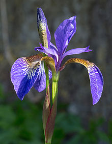
(image source: Wikipedia)
</span>
</div>


## Summarizing Scatter Plots

 * Recall: we summarize the distribution of **one continuous variable** with:
    * **center** (mean, median)
    * **spread** (standard deviation, IQR)
    * **shape** (symmetric/skewed, unimodal/bimodal/multimodal)
    * **unusual features** (gaps, outliers)

 * For **two continuous variables**, describe:
    * **direction** (positive association, negative association)
    * **shape** (linear, curved)
    * **unusual features** (gaps, outliers)


## Describe the relationship...

```{r, echo=TRUE, message=FALSE, fig.height = 4, fig.width=4}
ggplot() +
  geom_point(mapping = aes(x = petal_length, y = petal_width),
    data = iris) +
  ggtitle("Petal Length (cm) vs. Petal Width (cm)\nfor 150 Iris Flowers")
```

 * **direction** (positive association, negative association)
 * **shape** (linear, curved)
 * **unusual features** (gaps, outliers)

## Coloring by Species...

```{r, echo=TRUE, message=FALSE, fig.height = 3.75, fig.width=4}
ggplot() +
  geom_point(mapping = aes(x = petal_length, y = petal_width,
      color = species),
    data = iris) +
  ggtitle("Petal Length (cm) vs. Petal Width (cm)\nfor 150 Iris Flowers")
```

## Just the versicolor species

```{r, echo = TRUE, fig.height = 3.5, fig.width=4}
versicolor <- filter(iris, species == "versicolor")
ggplot() +
  geom_point(mapping = aes(x = petal_length, y = petal_width),
    data = versicolor) +
  ggtitle("Petal Length (cm) vs. Petal Width (cm)\nfor 150 Iris Flowers")
```

## Units I understand: 1 cm = 0.3937 in

```{r, echo = TRUE, eval = FALSE}
versicolor <- mutate(versicolor,
  petal_length_in = petal_length * 0.3937,
  petal_width_in = petal_width * 0.3937)
ggplot() +
  geom_point(mapping = aes(x = petal_length_in, y = petal_width_in),
    data = versicolor) +
  ggtitle("Petal Length (in) vs. Petal Width (in)")
```

<div class="col2">
```{r, echo = FALSE, fig.height = 3.25, fig.width=4}
ggplot() +
  geom_point(mapping = aes(x = petal_length, y = petal_width),
    data = versicolor) +
  ggtitle("Petal Length (cm) vs. Petal Width (cm)")
```

```{r, echo = FALSE, fig.height = 3.25, fig.width=4}
versicolor <- mutate(versicolor,
  petal_length_in = petal_length * 0.3937,
  petal_width_in = petal_width * 0.3937)
ggplot() +
  geom_point(mapping = aes(x = petal_length_in, y = petal_width_in),
    data = versicolor) +
  ggtitle("Petal Length (in) vs. Petal Width (in)")
```
</div>


## Shape of Plot Doesn't Depend on Units

```{r, echo = TRUE, eval = FALSE}
versicolor <- mutate(versicolor,
  z_score_length = (petal_length - mean(petal_length))/sd(petal_length),
  z_score_width = (petal_width - mean(petal_width))/sd(petal_width))
ggplot() +
  geom_point(mapping = aes(x = z_score_length, y = z_score_width),
    data = versicolor) +
  ggtitle("Petal Length vs. Petal Width")
```

<div class="col2">
```{r, echo = FALSE, fig.height = 3.25, fig.width=4}
ggplot() +
  geom_point(mapping = aes(x = petal_length, y = petal_width),
    data = versicolor) +
  ggtitle("Petal Length (cm) vs. Petal Width (cm)")
```

```{r, echo = FALSE, fig.height = 3.25, fig.width=4}
versicolor <- mutate(versicolor,
  z_score_length = (petal_length - mean(petal_length))/sd(petal_length),
  z_score_width = (petal_width - mean(petal_width))/sd(petal_width))
ggplot() +
  geom_point(mapping = aes(x = z_score_length, y = z_score_width),
    data = versicolor) +
  ggtitle("Petal Length vs. Petal Width")
```
</div>


## Correlation

* The (almost) average of products of $z$-scores: $r = \frac{\sum_{i=1}^n z^x_{i} z^y_{i}}{n - 1}$

<div class="col2">
```{r, echo = FALSE, fig.height = 3.5, fig.width=4}
versicolor <- mutate(versicolor,
  z_product_sign = ifelse((z_score_length * z_score_width) > 0, "Positive", "Negative"))

ggplot() +
  geom_point(mapping = aes(x = z_score_length, y = z_score_width, color = z_product_sign),
    data = versicolor) +
  geom_vline(xintercept = 0) +
  geom_hline(yintercept = 0) +
  scale_color_manual(values = c("orange", "blue")) +
  ggtitle("Petal Length vs. Petal Width")
```

</div>
* Using $z$-scores instead of original units means $-1 \leq r \leq 1$
* In this case, about 0.79

## Calculation in R

```{r, echo = TRUE}
cor(versicolor$petal_length, versicolor$petal_width)
```